Test
Mark D.
6 March 2018
# Week 1 activity
# lines starting with a '#' are comments

# import the csv data.
resp <- read.csv(here::here("01-CTT", "Bscored.csv"), stringsAsFactors = FALSE)

# calculate the score for each student (each row)
score <- apply(resp, 1, sum, na.rm = TRUE)

# calculate the item difficulty (each column)
itemdiff <- apply(resp, 2, mean, na.rm = TRUE) / apply(resp, 2, max, na.rm = TRUE)

# correlate each item column with the total score
disc <- apply(resp, 2, function(x) { cor(x, score - x, use = "complete.obs")})
Introduction
This is a test of English as Second Language for Grade 7 students. This is a pilot test for the purpose of evaluating test items for their psychometric properties so that a final test form can be constructed based on the results of this pilot test.
In total, 278 students took the test.
Classical Test Theory Item Statistics
discA <- as.integer(disc*100+0.5)  #these lines are for adding "*" and fixing two decimal places.
discB <- round(disc,2)
discB[(discA%%10)==0] <- paste(discB[(discA%%10)==0],"0",sep='')
discB[disc<0.2] <- paste("*",discB[disc<0.2],sep='')
itemstats <- data.frame(round(itemdiff,2),discB)
colnames(itemstats) <- c("Difficulty (%correct)","Discrimination(CTT)")
Item difficulty and discrimination
#itemstats
knitr::kable(itemstats,align = 'cc')| Difficulty (%correct) | Discrimination(CTT) | |
|---|---|---|
| B01 | 0.96 | *0.14 |
| B02 | 0.63 | 0.50 |
| B03 | 0.87 | 0.36 |
| B04 | 0.92 | 0.29 |
| B05 | 0.88 | 0.40 |
| B06 | 0.95 | *0.02 |
| B07 | 0.87 | 0.51 |
| B08 | 0.87 | 0.40 |
| B09 | 0.97 | 0.22 |
| B10 | 0.52 | 0.79 |
| B11 | 0.76 | 0.55 |
| B12 | 0.86 | 0.41 |
| B13 | 0.50 | *0.12 |
| B14 | 0.59 | 0.79 |
| B15 | 0.99 | *0.09 |
| B16 | 0.99 | *00 |
| B17 | 0.99 | *0.16 |
| B18 | 0.99 | 0.22 |
| B19 | 0.99 | *0.18 |
| B20 | 0.59 | 0.49 |
| B21 | 0.12 | *0.03 |
| B22 | 0.61 | 0.37 |
| B23 | 0.74 | 0.36 |
| B24 | 0.64 | 0.49 |
| B25 | 0.67 | 0.73 |
| B26 | 0.41 | 0.78 |
| B27 | 0.70 | 0.63 |
| B28 | 0.47 | 0.78 |
| B29 | 0.63 | 0.62 |
| B30 | 0.54 | *0.12 |
| B31 | 0.52 | 0.46 |
| B32 | 0.57 | *0.11 |
| B33 | 0.71 | 0.55 |
| B34 | 0.86 | 0.47 |
| B35 | 0.64 | 0.34 |
| B36 | 0.91 | 0.37 |
| B37 | 0.93 | 0.21 |
| B38 | 0.78 | 0.28 |
| B39 | 0.77 | 0.27 |
| B40 | 0.75 | *0.17 |
| B41 | 0.71 | 0.21 |
| B42 | 0.90 | 0.41 |
| B43 | 0.86 | 0.37 |
| B44 | 0.90 | 0.44 |
| B45 | 0.89 | 0.36 |
| B46 | 0.85 | 0.42 |
| B47 | 0.91 | 0.30 |
| B48 | 0.76 | 0.62 |
| B49 | 0.86 | 0.46 |
| B50 | 0.77 | 0.53 |
| B51 | 0.68 | 0.60 |
| B52 | 0.49 | 0.41 |
| B53 | 0.51 | 0.77 |
| B54 | 0.72 | 0.56 |
| B55 | 0.49 | 0.78 |
| B56 | 0.70 | 0.64 |
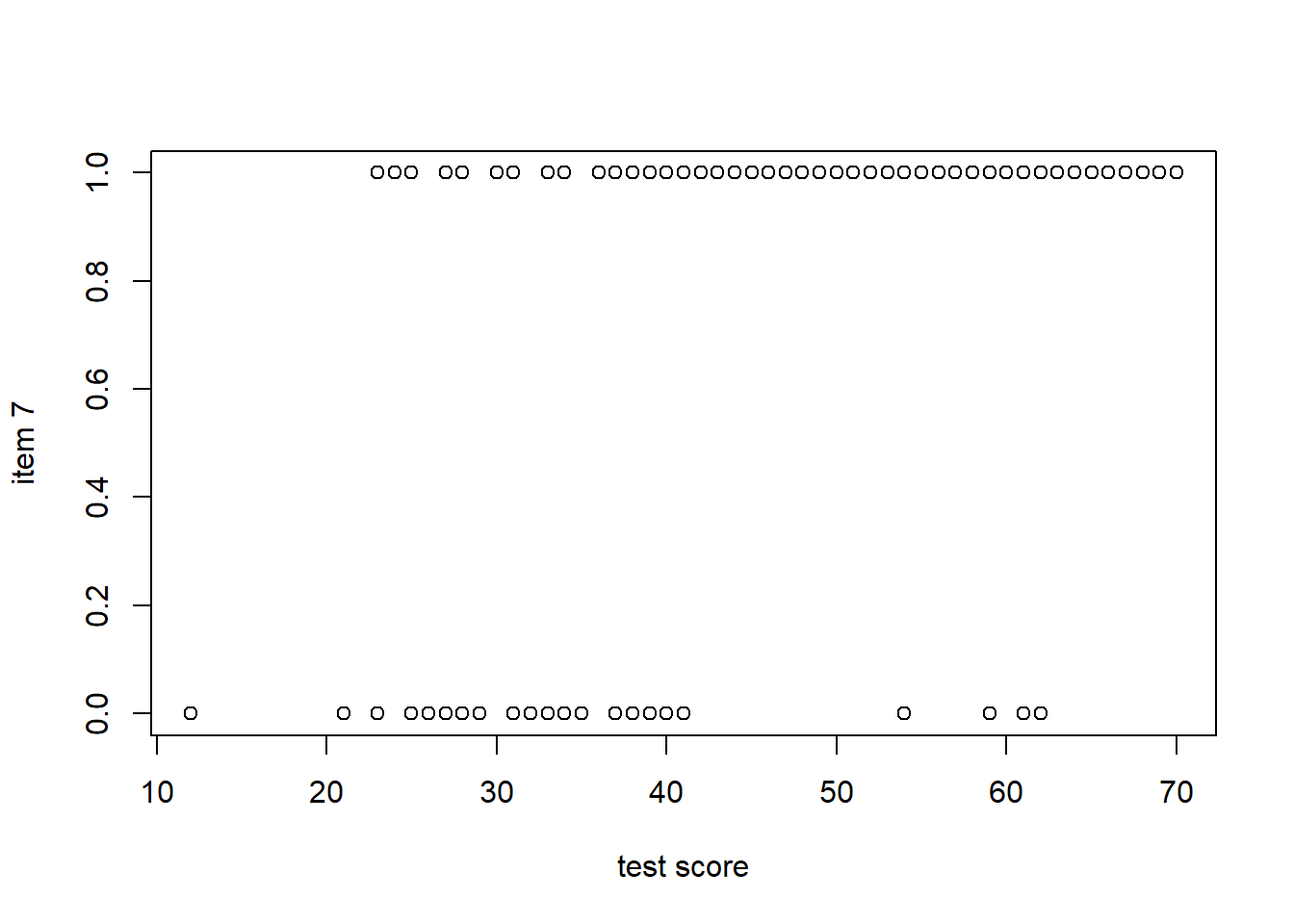
Plot of Item 7 score and total score
plot(score-resp[,7],resp[,7], xlab="test score",ylab = "item 7")